“No Match for a Good [IR] Blaster at Your Side, Kid”

On Saturday a few jumbled thoughts gelled together into an idea. First, I realized that we'd had quite a lot of fun blinking LEDs with our Raspberry Pi; then it connected that most IR emitters are nothing more than an LED, which the Pi should also be able to drive; finally, since Raspbian is a Linux distribution tuned for nerdy maker types, and Linux already has lots of support for working with IR, it should be pretty easy for us to build a Raspberry Pi contraption to control some of the electronics around the house.

Once I'd thought of this idea, I got really excited about it, since it would be a relatively simple extension of some of the work that we'd already done with the Pi but would perform a completely different kind of task: rather than making a simple visual display, we'd be using the Pi to communicate with other electronic devices already present in our home. As I mentioned last time, part of my interest in the Pi — aside from the sheer fun of messing around with exposed programmable I/O pins — is how working with it can help demystify some of the aura of magic that surrounds the hermetically-sealed, hyper-designed devices prevalent in the world today. Before we even started working, I got the chance to explain to my boys the basic idea of how an IR remote works: how a command on the remote (“power,” say) gets converted to a signal conveyed in a series of light pulses from the LED, how the TV performs this process in reverse to convert

light pulses to a command, and how different pulse patterns can be used to communicate different commands to the target device. Add to that the cool factor of seeing something that we soldered together on the kitchen table control a sophisticated piece of consumer electronics, and it was clear that we had a winner of a project on our hands!

For this project I elected to use the same “hello Pi” LED circuit from our previous experiments, which is simply the emitter LED with a current limiting resistor, 100 Ω this time as I wanted minimal current restriction:

Depending on the emitter you're using you might find this results in fairly limited range, and several folks on the web suggest using a transistor circuit to drive the LED from a higher-current power source than the Pi's GPIO pins. It turns out I had a low power emitter/detector pair on hand (from RadioShack!), and, since I wasn't especially concerned with range, we went with the simple route.

At first I thought about programming the emitter directly, but a blog post or two quickly dissuaded me from this idea. It turns out that driving a 38kHz signal from an unsupported user program is difficult or impossible in Linux, so rather than get stuck on fighting with that bit, I elected to take advantage of the vast resources afforded by the community, which had already solved this problem in the form of LIRC, the Linux IR Remote Control project. Not only is there excellent support for IR in general on Linux, some kind soul had already concocted an LIRC driver that works with the Pi's GPIO pins, which is available in the latest Raspbian release with a simple

    sudo apt-get install lirc

to install both LIRC itself and the lirc_rpi driver. The driver allows you to wire simple, readily available IR components to the Pi's GPIO header for a quick, easy, and cheap programmable IR device.

Next we needed to solder the emitter to its wiring. This time I had Asher (7) do the soldering for us: I held the joints, he heated them, and I applied the solder. With some strong warnings and lots of careful guidance, he was able to desolder one joint — we repurposed a wiring harness from our last project — and solder the three new connections we needed without burning himself, me, his brother, the house, or anything else that I could detect. Success! His mother tells me that this experience thrilled and encouraged him, which is the best possible outcome from a project like this: delighting and empowering someone else.

Getting LIRC set up on the Pi is fairly easy thanks to this guide, just make sure you adjust the gpio_out_pin arguments to match the pin you're planning to connect the emitter to (in our case GPIO 17, i.e. physical pin 11). A couple of additional notes on working with LIRC:

• the version of LIRC packaged in Raspbian is fairly old, so some features mentioned in the LIRC documentation do not work. One specific gotcha is that the support for multiple config files in /etc/lirc/lircd.conf.d/ isn't implemented in this version, so if you want to emulate multiple devices you'll need to combine the device definitions yourself. The include directive is implemented, which is what I used to do this.
• LIRC's configuration parser is pretty picky — for example, comment lines cannot begin with leading whitespace — and ferreting out configuration problems can be a challenge when the daemon is started automatically at boot. I found it helpful to run LIRC in the foreground (lircd -n) while I messed with the conf files until it was happy.
• With the default install, restarting LIRC (/etc/init.d/lirc restart or stop then start) would not bring things back up correctly: restarting left irsend unable to find the running lircd. I'm sure this is a simple configuration mismatch somewhere, but my low-tech solution was to simply reboot the Pi when I got the configuration the way I wanted it.

Fiddling around with config files isn't very engaging, so I took over the next bit: finding remote control definition files for the remotes we wanted to emulate. The LIRC project has collected a large number of device definitions from users around the web, and we were able to find a direct match for the remote control for our TV. After some experimentation we also found a remote definition that would talk to the receiver using a slightly different model number than is printed on the actual remote. LIRC also supports reading signal codes using a receiver circuit, but we have not tried that yet.

Now the moment of truth: I held the emitter so it was pointed at the TV while Asher ran the command

    irsend SEND_ONCE samsung KEY_POWER

from the terminal. We both had huge grins as the TV's standby indicator light winked off while it went through its power up sequence and finally ignited the panel. We goofed around running a few more commands at the TV and receiver before declaring this project a success.

What are we going to do next with our IR blaster? Who knows, although I must admit to being tempted by this kit from Adafruit, which, while not a Raspberry Pi project, connects to these same concepts and provides excellent guidance on basic electronics skills. But even if nothing else comes of it, I'm satisfied at completing another project that engaged my children's imagination, empowered them with new knowledge, and encouraged them to explore their interests courageously.

Deck the Halls with Raspberry Pi

I'm continually on the lookout for ways to connect with my children, especially my eldest whose natural interests seem to be rather different from mine. Going into parenthood I expected to engage my children easily over interesting science and technology subjects. It's certainly in their blood: their mother is a scientist and I am a software developer and general tinkerer. Reality has, as it so often does, proven less straightforward, more ambiguous. I'm sure there are many causes and influences, but one obvious theme concerns the sheer scope and pace of technological advancement since my own childhood. My first computer — a Commodore VIC-20 — seems hopelessly primitive next to the bewildering assortment of hypernetworked computing devices my children see their grandparents carry in a pocket.

While I struggle to identify the essential difference in our experiences, I suspect that part of what has changed is that my children aren't interested in computers as such the way I was. They beg to get tablet time to watch videos or play an online game, but everything they experience is professionally produced and logically ordered, with all the rough edges and sharp corners neatly rounded off into beautiful, pleasing curves.

My formative experiences were quite different. To them, using a VIC-20 would seem like a pathetically empty experience by contrast with the devices they're used to. No slick fade ins to carefully crafted notifications blending seamlessly with expensive, highly tuned interfaces to precisely-defined destinations. Even turning the VIC on felt like a primordial act, the massive, honest-to-goodness SPST coursing with power that flowed past your finger and off toward unknown and terrifying adventures. Yet even after that nothing much happened, nothing but a blinking blue expectancy, a half imagined whisper of potential. But of course that was the magic of it: you didn't turn on a VIC so much for what it could already do; you turned it on because of what you could make it do, for all of the wonderful creative possibilities its existence suggested. While the intervening decades have brought transformative advancements in the capabilities of our information technologies, the exploratory capacity, this frontier-like horizon that was the VIC's foremost asset, can become lost in the well-worn ruts of design.

This helps explain why, on a whim shortly before Christmas, I packed my boys into the truck and headed over to Micro Center to pick up a Raspberry Pi 2. The actual purchase jarred me a little by its contrast with my childhood memories, the agonized handwringing and haggling over the purchase of some part or accessory, which cost much more and did much less than the tiny little box the three of us carried out of the store. But there's something compelling about these little devices that manages to recapture some of the joy of possibility that hooked me on computing in the first place. Perhaps it's the physical board itself, so unlike a phone or tablet, with its rough circuit board edges crammed to bursting with connectors, sharp solder points and interface pins sticking weirdly out of every surface. Or maybe it's the surprising scale that delights, the wonder that something so small can do so much. It could be all those I/O pins practically begging to be hooked up to lights, sensors, and other gizmos. Whatever the reason, there is something about this device that manages to break through the conventional abstractions to reawaken wonder, the possibility of possibility.

Our first Pi project was a humble one: we hooked up a software-controlled LED, which is pretty much the equivalent of “hello, world!” for the Raspberry Pi.

As with most tech projects, even something as seemingly simple as a light on a switch requires daunting amounts of paraphernalia, patience, and time. For us, though, that was part of the fun: trucking around town on some fool idea of dad's, rummaging in obscure corners of the basement closet for resistors, LEDs, and bits of wire, the improbability of seeing the Pi driving an HDTV, fidgeting while the adults scratched their heads over some technical snag.

To get started on your own Pi adventure, you'll need a Raspberry Pi board [1], a micro SD card with the Raspbian OS installed [2], a micro USB power source (such as a phone charger), a screen with HDMI or composite video inputs and appropriate cabling, and a USB keyboard and mouse. (Whew!) Test booting the Pi up to make sure you have a working setup; there is nothing quite like the frustration of getting stuck for an hour and then discovering a bad cable.

For the LED mini project you'll need a few more parts: an LED, a current limiting resistor, some wire, and jumpers to attach to the Pi's GPIO pins. If you've got an old desktop computer lying around, you can scrounge the LED, wire, and jumpers from its indicator lights. And you should probably get yourself a breadboard and jumper wires for it, but for this simple circuit I was content to solder the components directly.

There are many excellent showcase and tutorial sites out there to spur project ideas and help you get going. We headed over to Gordon's Projects Single LED tutorial, which takes you through the steps of getting the LED connected; he does a nice job of breaking the narrative into digestible chunks and interspersing concept explanations to help orient beginners. (I still find the multiplicity of GPIO pin numbering and addressing schemes confusing, but I don't at all fault Gordon for that). Following his instructions we quickly had the LED wired up and connected to our Pi, which we then tested with the gpio utility, prepackaged with Raspbian Jessie, that can be used to communicate with the Pi's GPIO bus. From the console we ran these commands:

The pattern of these commands is gpio <subcommand> <pin> <value>, so the first command translates roughly to “set GPIO user pin 0 to output mode.” GPIO pins can be configured for input or output, depending on whether you are reading from a sensor or driving a motor or LED. Once the pin was configured, we used the second command to turn the LED on and the third to turn it off.

With that working, the obvious next step was to control the LED using Python. There are several Python libraries for interacting with GPIO; we used GPIO Zero, as documented in this tutorial by the Raspberry Pi Foundation. Here's the same sequence of commands as above, but this time using Python:

Instead of interacting directly with the bus, GPIO Zero provides a number of utility classes for dealing with commonly used devices; unsurprisingly the LED class is used to control an LED. The class encapsulates the fact that the LED is an output device and configures the pin to output mode for us when we instantiate it.

Why 17? That's the pin number according to the GPIO numbering scheme, which is equivalent to wiringPi user pin 0 (hence the 0 in the gpio commands above); both refer to physical pin 11 on the board. Ahem.

Pin numbers aside, our next challenge was to make the LED blink, which we accomplished with this simple Python script:

By this point I'd pretty much exhausted the boys' attention capacity, so we got out coloring supplies and drew some Christmas trees. Taking the LED we'd wired up and pushing it through the cardboard yielded a simple Raspberry Pi-powered Christmas display! Over the next few days I added three additional LEDs and some programming to expand the display:

So was this project successful in establishing a deeper interest in the workings of computing technology with my children? Time will tell, but one gain afforded by our little hack is that it has given us a platform to talk about how other things work. They have many small toys that use microcontrollers to control lights, drive motors, react to button presses, and play sounds and music; seeing the construction of this simple project has let me draw their attention to the basic workings of such devices via analogy to our Pi tree. At least in a small way I think they are beginning to understand that electronic devices are not magic and to see how we might build simple devices like the toys they're used to.

My next project? I'm working on building a Raspberry Pi-based geotagger for my Nikon DSLR; I'll be documenting the steps in a series of posts over the coming weeks, so stay tuned!

* * *

Resources

• source code for our Christmas tree display
• Raspberry Pi Learning Resources from the Raspberry Pi Foundation
• GPIO Zero library documentation
• Gordon's Projects GPIO Examples
• Gadgetoid has a nice interactive pinout guide

---

[1]	I recommend the Raspberry Pi 2 Model B, but the older models should work as well. Avoid the Raspberry Pi Zero when you're starting out: the Zero is incredibly cool and tiny, but it is less user-friendly than the other models as it lacks some of their connectivity conveniences.

[2]	There are serveral other OS options for the Pi, and you should obviously go play around with all of them. The examples in this post assume the presence of several supporting tools and libraries that are preloaded on Raspbian Jessie.

Of Dictionaries and Analysis

I greatly enjoyed reading Andrew Kuchling's Beautiful Code article “Python's Dictionary Implementation: Being All Things to All People,” [1] in which Kuchling explores some of the implementation details of what is arguably CPython's most important data structure: the dict. While these implementation details themselves are fascinating, the article offers a deft illumination of the thought process that led to the selection of a given implementation over its alternatives. The lessons here are not just for open source hackers working on the performance-critical portions of a popular language: they offer sound process guidance to anyone needing to make wise choices in the face of conflicting needs and trade-offs when building any kind of software.

Kuchling summarizes his main thesis about halfway through the article:

When trying to be all things to all people — a time- and memory-efficient data type for Python users, an internal data structure used as part of the interpreter's implementation, and a readable and maintainable code base for Python's developers — it's necessary to complicate a pure, theoretically elegant implementation with special-case code for particular cases… but not too much.

The brilliance of the article rests on how Kuchling shows the available trade-offs for a given problem explicitly, always couching them in reference to those user groups and their real-world needs. It's interesting as a postmortem, but also offers a valuable blueprint for structuring design processes such that compromises get debated on their specific, explicitly articulated merits and shortcomings rather than on hidden assumptions, preferences, and biases. Once the options are on the table, it becomes possible to consider their strengths and weaknesses in light of the needs of affected users rather than having to rely solely on theoretical or aesthetic considerations.

With that in mind, here are some specific lessons we can draw from the article about how to structure the process of analyzing potential software solutions.

Lesson 1: Maintainability Matters, Therefore Maintainers Matter

An important but subtle take away from Kuchling's thesis is that developers form one of the user groups with a stake in the outcome, and that therefore code readability and maintainability constitute legitimate, first-order user concerns that deserve weighted consideration alongside the needs of other user groups. Although Kuchling doesn't provide specific examples demonstrating this trade-off in action, this idea forms a theme woven throughout the entire discussion: unless you have a compelling, measured reason not to, prefer simplicity.

This can be challenging conversation to have, especially in commercial contexts with their strong emphasis on feature delivery and satisfying client user demands. A mechanism we use to allow compromise on this front, which we can call the “maintainability gradient,” suggests that changes that have broader reach or usage mandate a higher level of scrutiny with respect to complexity and maintainability. When considering a client request, for each solution under discussion the development team offers an assessment of its maintainability: the solution's inherent complexity, the ease or difficulty of implementing it within the framework and underlying assumptions of the existing platform, especially under time constraints, and the likelihood that we will be required to tinker with it after delivery. This becomes one of the inputs that helps us determine where in the layered architecture a given solution will be allowed:

Figure 1: Our layered architecture. The top of the stack is the most-specific, least-shared code, while the bottom layers are most shared.

In this context, our maintainability gradient provides guidance about where complication is acceptable and where it is not: while we always strive to create simple solutions, if an end user insists on something complicated or messy, it is shunted to client-specific code where its impact on the platform can be minimized and contained. Conversely, proposed additions to the core platform must meet a higher standard of maintainability: does this change fit within the existing context of the platform? Can it be implemented simply and readably?

Note that this is not an excuse to do slipshod work, even in obscure cul-de-sacs of custom code. Quite the opposite: this approach empowers developers to do great work everywhere within the context of a resource-constrained commercial enterprise. If a solution can't be maintainably generalized under current constraints, we can implement a smaller, specific version where the solution is easier to isolate. We don't always get the trade-off right, but this architecture gives us an axis of compromise that allows maintainability to have a voice in the conversation.

Lesson 2: Whom Do You Serve?

Another key design process lesson from Kuchling's article is that it is imperative to understand users and their needs, and to evaluate proposed solutions in light of those needs. Concretely, this means

1. listing each alternative explicitly
2. describing the characteristics of each solution relative to each user group
3. choosing the solution that is the best compromise among the various alternatives

The short section on handling hash collisions in the article illustrates this process nicely. The problem is this: when implementing a hash table, what do we do when two keys inevitably hash to the same slot?

One option is to use chaining: instead of single values, each slot holds a list of values with the same hash. CPython does not do this “because creating linked lists would require allocating memory for each list item, a relatively slow operation.” In other words, CPython does not use chaining because this solution fails to meet the needs of at least two of the important user groups identified earlier: end-users of Python needing an efficient mapping data structure, and the language implementors who need an efficient platform on which to build objects, modules, and functions.

The next option up for consideration is linear probing: if a needed hash slot $i$ is occupied, examine $i+1$, $i+2$, etc. This solution is quite simple to implement, but again CPython does not use it. Why not? “Many programs use consecutive integers as keys,” which, due to how CPython hashes integers, consume contiguous blocks of the hash table that are inefficient for linear probing. Having identified the performance characteristics of this solution explicitly, it is easy to see the trade-offs being made here and the user groups affected by those trade-offs: linear probing is simple to implement — a boon for the maintainers — but that simplicity yields a solution that does not serve the performance needs of the language implementors or end-users very well.

This analysis is predicated on both understanding who the users are and what their usage patterns look like while simultaneously understanding the spectrum of available solutions considered in light of the needs of those various user groups. In the end, CPython's hash collision resolution algorithm is a pragmatic compromise, guided by experimentation, measurement, and feedback, that concedes a little code complexity in exchange for good performance characteristics in the real world.

Lesson 3: … but not too much

My favorite optimization that Kuchling describes is a complexity/performance trade-off. The dilemma is this: how can the dict implementation serve a general audience — by handling non-string keys, rich comparison operators, and possible exceptions — while also offering good performance for the huge swath of dict usages with exclusively string keys, such as those that underlie the implementation of classes, modules, and functions?

One approach would be to implement separate classes: a specialized, string-only dict optimized for high-performance for this use case along with a more general purpose implementation for regular use. In fact this is exactly what Jython, the Python implementation that runs on the JVM, does: it utilizes Java's java.util.HashMap as the basis for the dict implementation for general purpose use but employs a separate, optimized class to handle the performance-sensitive language implementation bits.

CPython instead uses a single implementation but employs two different lookup functions. By default, dicts are assumed to contain only string keys, and since many of the complexities and failure modes that arise when comparing two arbitrary objects are impossible when comparing two strings, the default lookup function can be optimized to eliminate checks for cases or errors that simply cannot happen. The implementation is a classic use of indirection that relies on a simple function pointer: if an arbitrary, non-string object is searched for or inserted into a dict instance, the search function pointer for that instance is updated to reference the slower but more general purpose lookup implementation that can handle the added complexities concomitant with comparing arbitrary objects.

This example beautifully illuminates a pragmatic, “not too much” compromise that serves its various users well. For the language implementors, the solution provides an important performance boost for lookups in classes and modules and passing of keyword arguments to functions, all of which are exclusively string- keyed and are the most frequent operations in a running Python program. It is also fairly simple, easy to understand, and is likely less code than a two-class solution would be. This in turn helps minimize the potential for implementation drift and maintains the “fits in your head” quality valued by the Python community.

The compromise also serves end users very well: string-keyed dicts are very common in many applications, so end users reap a double benefit: attribute lookups and function calls are faster, and, as an added bonus, portions of their systems that rely on string-keyed dicts are also sped up.

* * *

[1]	I couldn't find the article online except at Safari (free trial available).

Building a Unicode .format Nanny with Python's AST

Detecting problematic .format calls quickly and painlessly using Python's powerful ast module. Follow along by downloading the Jupyter notebook of this post!

The issue: where I work, we are still a Python 2 shop owing to technical debt and legacy dependencies. Since Python 2's default string type is a byte sequence, painful encoding-related problems surface in our applications from time to time. A fairly typical example runs something like this: a developer writes some code to format data into a string, using the convenient and powerful .format method supported by all string objects:

In [1]:

def pretty_format(some_data):
    return 'Hello, {}!'.format(some_data)

Through the course of our exhaustive testing, we prove that this function is correct over a wide range of inputs:

In [2]:

print pretty_format('world')

Hello, world!

The code ships. Months pass without incident, our pretty_format routine prettily formatting every bit of data thrown its way. Lulled into complacency through enjoyment of our apparent success, we move on to other tasks. One day, everything comes to a screeching halt as, completely unprepared, we receive one of the most dreaded error messages in all of software development:

UnicodeDecodeError: 'ascii' codec can't decode byte 0xc3 in position 8: ordinal not in range(128)

What happened? Why did code that worked flawlessly for months suddenly detonate, without warning, without mercy?

Much of the data that flows through this format template and others like it is simple ASCII-valued information: dates, addresses, phone numbers, and the like. Having used Python 2 for many years, we are habituated to spell strings, including our template formatting strings, using the simple single quote

'a typical string'

What happens, though, when our user data contains an accented character or other non-ASCII symbol?

In [3]:

full_name = u'Ariadne Éowyn'
print pretty_format(full_name)

---------------------------------------------------------------------------
UnicodeEncodeError                        Traceback (most recent call last)
<ipython-input-3-3d955b7228e5> in <module>()
      1 full_name = u'Ariadne Éowyn'
----> 2 print pretty_format(full_name)

<ipython-input-1-51c87778ff71> in pretty_format(some_data)
      1 def pretty_format(some_data):
----> 2     return 'Hello, {}!'.format(some_data)

UnicodeEncodeError: 'ascii' codec can't encode character u'\xc9' in position 8: ordinal not in range(128)

Boom! Python detects the mismatch between the byte string template and the Unicode data containing some multi-byte characters that simply cannot be represented directly in the target format, ASCII. In other words, Python is refusing to guess what we want: do we prefer a binary expansion, and, if so, in what encoding? Should the accent characters simply be dropped? Do we want unexpected symbols to be translated into ASCII error characters? Python has no way of knowing which of these options is appropriate to the present situation, so it takes the only reasonable course and raises an exception.

Many encoding issues can be quite challenging to reconcile, but this case is rather simple: if the format string is specified in Unicode format — rather than as a plain byte string — this entire class of problem would be avoided:

In [4]:

def pretty_format(some_data):
    # Unicode template prepares this routine to handle non-ASCII symbols
    return u'Hello, {}!'.format(some_data)

print pretty_format(full_name)

Hello, Ariadne Éowyn!

But how do we know where the problematic calls to .format are lurking in our code base without waiting for the next error to occur? Is there a way we could find these calls proactively, eliminating them from the system before they wreak havoc on our application?

A brief diversion, or Now you have two problems¶

When I first mentioned the idea of automatically detecting problematic .format calls to a coworker, he immediately quipped back “have fun writing that regex!” Before we look at a more powerful and reliable alternative, let's take a moment to examine his intuition and understand why we might not want to use regular expressions for this task.

At first glance, regular expressions seem reasonably well suited to this job: what we're looking for are substrings of a given string — that is, parts of a Python source file — containing a certain pattern. Indeed it is fairly easy to construct a first cut at a regular expression for this. Here is mine, including a bunch of explanatory comments:

In [5]:

import re

# a first draft regular expression for detecting 
# problematic .format calls
pattern = re.compile(r'''
    (?x)        # turn on verbose regex mode
    
    (?<!u)      # ignore matches that start with a u
    
    '           # match ', followed by 
    [^']*       # any number of non-' characters,
    '           # followed by '
    
    \.format    # only if the string is followed by a
                # call to .format
    ''')

This appears to work well for some simple cases:

In [6]:

def is_problem(s):
    return bool(pattern.search(s))

print is_problem("message = 'Hello, world!'")
print is_problem("message = 'Hello, {}!'.format")
print is_problem("message = u'Hello, {}!'.format")

False
True
False

but will fail for many, many others. What if the code we're examining uses double quoted strings? Or multiline strings? Does the regular expression we've concocted handle continuation lines correctly? Backslash escapes? Comments? Here are just a few example cases that our regex will not report correcly:

'another {}string' \
    .format

"now you're just" \
'bein\' {}annoyin\''.format(u'seriously ')

# 'ignore me'.format

Just for fun, here are a few more: what happens if we use the Python parser's string combination feature?

In [7]:

# a false positive
is_problem("""
    u'this ' 'and this are the same string{}'.format
""")

Out[7]:

True

Or if you get in your time machine and import Unicode literals?

In [8]:

# another false positive
is_problem("""
    from __future__ import unicode_literals
    
    'Unicode masquerading as {}'.format
""")

Out[8]:

True

To be effective, our source examination tool needs to handle all these cases and more so that team members will trust the feedback they are receiving: we don't want to create alarm fatigue by producing false or spurious warnings. On the other hand, there are many edge cases and difficult combinations that will require a complicated parser solution to handle correctly.

Notice, though, that Python's own parser already deals with all of these difficulties when interpreting our source code! Since the Python language and community emphasize openness and introspection, it will probably come as no surprise that this machinery is exposed and available to Python programs. Using the ast module, we can transform arbitrary Python source into a tree representation, with all of the aforementioned parsing complexities already handled for us. Our task then becomes much simpler: we merely need to inspect this tree and report any instances of calls to .format that are made on byte strings.

What's an AST?¶

An abstract syntax tree (AST) is an object representation of the syntactic parts of a program and of the relationship between those parts. If we have some program fragment,

for little_one in ['Asher', 'Ansel', 'Ariadne', 'Andromeda']:
    name_complexity = len(little_one)
    print name_complexity

we can observe that there is a lot going on in even a relatively simple construct like this one:

• the entire construct is a logical unit with respect to the other statements that may surround it. For example, moving this statement around will not change its internal semantics (although moving it may still affect the semantics of the program around it)
• the statement itself consists of 3 components: the iterable that supplies the values for the loop, the assignment target, and the loop body, which is in turn composed of multiple statements
• each of the parts have a specific relationship to the others that is communicated by the source code. This relationship forms part of the semantic structure of the statement: if we were to move the print call back 4 spaces, we would alter the relationship of the parts to each other and therefore the semantics of the entire statement:

for little_one in ['Asher', 'Ansel', 'Ariadne', 'Andromeda']:
    name_complexity = len(little_one)
print name_complexity

An AST captures these nuances in object form. In an AST representation, nodes model individual constructs in the program, drawn from the set of all available constructs defined by the language. In Python, for example, we have node types representing Module, For, Name, and Str. Each node captures both the type of construct being represented and the details of a particular instance: the Name class represents all possible variable usages, while a particular instance of Name in an AST will include the specific name used at a given point in a program and whether that name is being read from or written to.

Let's take a look at the AST representation of this for loop:

In [9]:

import ast
tree = ast.parse("""

for little_one in ['Asher', 'Ansel', 'Ariadne', 'Andromeda']:
    name_complexity = len(little_one)
    print name_complexity

""")

print ast.dump(tree)[:92] + u'…'

Module(body=[For(target=Name(id='little_one', ctx=Store()), iter=List(elts=[Str(s='Asher'), …

First we parse the source text into a tree representation, then ask the ast module to dump that tree structure back out as text. Since the output of ast.dump can be somewhat difficult to read, I've indented this particular trace by hand to reveal the relationship structure of the tree:

Module(body=[
  For(
    target=Name(id='little_one', ctx=Store()), 
    iter=List(
      elts=[Str(s='Asher'), Str(s='Ansel'), 
            Str(s='Ariadne'), Str(s='Andromeda')], 
      ctx=Load()), 
    body=[
      Assign(
        targets=[Name(id='name_complexity', ctx=Store())], 
        value=Call(
          func=Name(id='len', ctx=Load()), 
          args=[Name(id='little_one', ctx=Load())], 
          keywords=[], 
          starargs=None, 
          kwargs=None)), 
      Print(
        dest=None, 
        values=[Name(id='name_complexity', ctx=Load())], 
        nl=True)], 
    orelse=[]
  )
])

The Module object is the outermost container for our code. It corresponds to a .py file and contains a single attribute, body, that contains the list of statements — imports, assignments, function and class definitions, etc. — that make up the module. For this simple example, the module body contains one element: our for loop.

With a little squinting, you can see the two body statements contained within the for loop attached to the For node's body attribute: Assign and Print. This brings the total number of direct children of the For node to four: a List node as its iterable, a Name node as its target, and the Assign and Print nodes making up its body. The List, Assign, and Print nodes each have their own children representing the string literals that make up the list, both sides of the assignment statement, and the values we wish to print.

Given this general introduction to Python's AST, here are two examples illuminating what our .format nanny will be looking for; first is a case we want to alert the user about:

In [10]:

ast.dump(ast.parse("'a {}string'.format"))

Out[10]:

"Module(body=[Expr(value=Attribute(value=Str(s='a {}string'), attr='format', ctx=Load()))])"

followed by an acceptable spelling that should produce no warning:

In [11]:

ast.dump(ast.parse("u'a {}string'.format"))

Out[11]:

"Module(body=[Expr(value=Attribute(value=Str(s=u'a {}string'), attr='format', ctx=Load()))])"

Translating this into a textual description lets us refine the problem statement we formulated earlier: we are looking for Attribute nodes with an attr of 'format' and whose value is a Str node. If that Str node's s attribute starts with a ' and not a u, we have found a problematic spelling and should warn the user.

Stop and ponder this for a moment. Notice how we've gone from a definite but ambiguous notion of what we wanted to a simple, precise, and implementable description that leverages the transformation of source text into a tree representation.

Visiting .format¶

Python's ast module provides a tree traversal framework for working with ASTs that is based on the Visitor pattern. For each node type, a custom traverser defines a method corresponding to that type that will be invoked whenever the traversal encounters such a node. For example, here's the basic template for working with Attribute nodes:

class MyVisitor(ast.NodeVisitor):
    def visit_Attribute(self, node):
        # do something with Attribute nodes

Let's do some exploratory coding. We've already seen the basic structure of the Attribute nodes we're looking for, but what else is available to us as we're traversing an AST?

In [12]:

tree = ast.parse("""

'Hello, {}!'.format('world')

pi = math.pi

""")

In [13]:

class AttributeInspector(ast.NodeVisitor):
    def visit_Attribute(self, node):
        print node.__dict__
        print node.value.__dict__
        print

AttributeInspector().visit(tree)

{'col_offset': 0, 'ctx': <_ast.Load object at 0x7ff178b71a10>, 'attr': 'format', 'value': <_ast.Str object at 0x7ff15bffe910>, 'lineno': 3}
{'s': 'Hello, {}!', 'lineno': 3, 'col_offset': 0}

{'col_offset': 5, 'ctx': <_ast.Load object at 0x7ff178b71a10>, 'attr': 'pi', 'value': <_ast.Name object at 0x7ff15bffec10>, 'lineno': 5}
{'ctx': <_ast.Load object at 0x7ff178b71a10>, 'id': 'math', 'col_offset': 5, 'lineno': 5}

This little class simply prints the instance dictionaries for each Attribute node in the tree along with that of its value attribute. I often use this trick (print obj.__dict__) when exploring a problem to help me understand the attributes and capabilities of unknown objects. For this particular problem, our inspector has revealed that each node type has a different set of attributes defined on it and given us clues to help us advance to a solution.

As expected, there are two Attribute nodes in our little example program, corresponding to the .format and .pi references in the source. We saw earlier that we are specifically looking for nodes with an attr of 'format', and our little test class revealed another bit of useful data: the line number on which the attribute access appears in the source, which will be useful information to provide back to the user.

Our tiny Visitor implementation has already solved the first part of our problem: finding Attribute nodes in the source. All that remains is to filter down to .format nodes and check the value attribute of each. Here is the rest of the implementation:

In [14]:

class FormatVisitor(ast.NodeVisitor):
    def visit_Attribute(self, node):
        if node.attr == 'format':
            _str = repr(node.value.s)

            if _str[0] != 'u':
                print u'{}: {}'.format(node.lineno, _str)

With just a handful of lines of Python, we have created a program that meets the goals we set out above. This solution harnesses the full power of Python's exposed parser machinery, which allows our code to express a very high level solution with a minimum of syntactic overhead. Run on our example above, it points out that line 3 of the source contains a problematic spelling:

In [15]:

FormatVisitor().visit(tree)

3: 'Hello, {}!'

while source with an acceptable spelling yields no warnings:

In [16]:

tree = ast.parse("""u'Hello, {}!'.format('world')""")
FormatVisitor().visit(tree)

Here is a complex example that demonstrates several of our tricky cases from earlier, including a split string, continuation line, and even a parenthesized expression!

In [17]:

source = """

('Hello, '
    '{}!') \
.format('world')

"""

tree = ast.parse(source)
FormatVisitor().visit(tree)

3: 'Hello, {}!'

The same source but with corrected strings eliminates the warning:

In [18]:

source = source.replace("('", "(u'")
tree = ast.parse(source)
FormatVisitor().visit(tree)

Even the __future__ import case is handled correctly with no extra effort on our part!

In [19]:

tree = ast.parse("""

from __future__ import unicode_literals
'Hello, {}!'.format('world')

""")
FormatVisitor().visit(tree)

Looking back, looking ahead¶

Thanks for joining me in this tour of a lesser-used corner of the Python standard library. In my shop, we now use a Git commit hook based on these ideas to help detect these sorts of encoding problems before they even make it into the source tree. Figuring out how to build the hook was a fun exploration with a pragmatic result, and I hope that you have enjoyed walking through it with me and that you learned something along the way!

If you'd like to learn more, here are a few resources to continue your exploration:

• Green Tree Snakes is Thomas Kluyver's introduction to the AST, billed as “the missing Python AST docs”
• The ast module documentation contains a grammar specification and module reference
• Andreas Dewes presented a static analysis tool at PyCon 2015 based on the AST
• Hy implements a Lisp interpreter in Python and makes extensive use of the AST

Clean and Green: Pragmatic Architecture Patterns

Thanks to everyone who came to my PyTennessee 2015 talk, Clean and Green: Pragmatic Architecture Patterns! 

• screencast of the presentation
• the slides include additional material we did not have time to cover

If you are interested in learning more about the Clean Architecture, the following resources provide a wealth of information about the theory and practice:

• Brandon Rhodes, The Clean Architecture in Python, (slides, video)
• Uncle Bob Martin, The Clean Architecture, (and reactions)
• Gary Bernhardt, Boundaries
• J B Rainsberger, Integrated Tests are a Scam

A Monte Carlo Example in Python

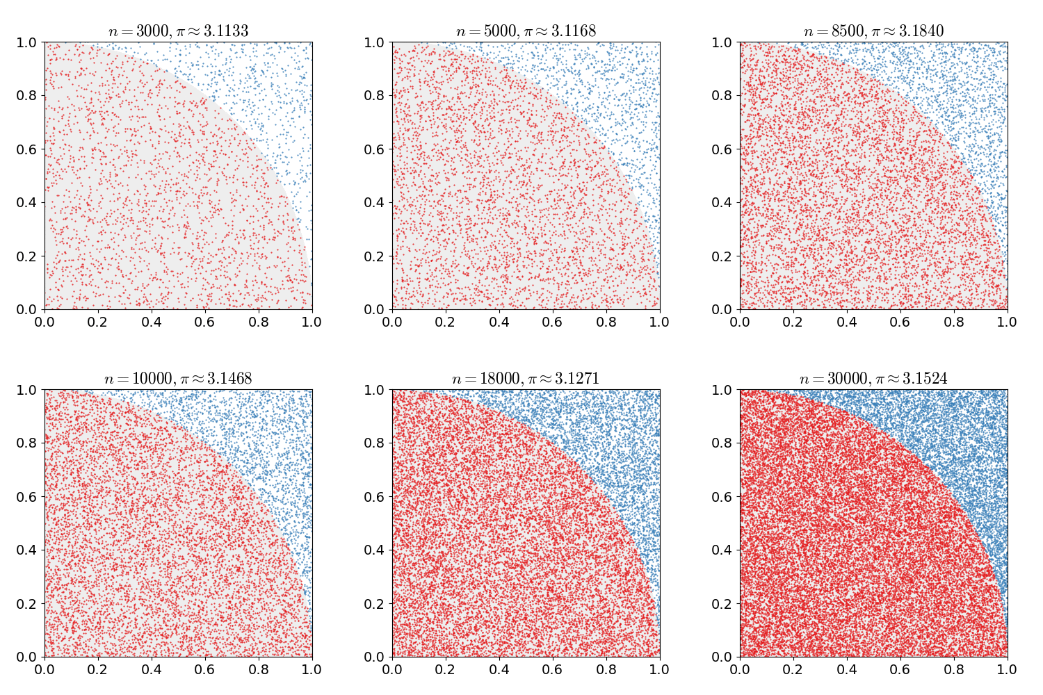
While reading about Monte Carlo methods, I came across this fascinating image created by Caitlin Jo Ramsey:

This plot illustrates a Monte Carlo method for determining π, which I immediately determined to try to reproduce in Python. This post is an IPython Notebook demonstrating how to perform this method using modern Python tools and techniques.

Caveat emptor: Monte Carlo methods are not the best technique for generating approximations of π, so if that's what you are interested in, check out Wikipedia's π page or search around for implementations in your favorite language. On the other hand, the algorithm does offer a nice introduction to Monte Carlo methods as it is

• simple
• reasonably intuitive
• easily verifiable
• fast enough

Let's get started!

Monte Carlo?¶

What are Monte Carlo methods? A Monte Carlo method is a probabilistic algorithm that relies on random sampling rather than strict determinism to obtain its result. Monte Carlo methods are useful in many fields, particularly when the complexity of the problem in question renders deterministic solutions infeasible.

The example above uses a Monte Carlo method for approximating π. Here's how it works: picture the unit square and the unit circle, with the center of the circle at the origin. Let \(r = 1.0\) be both the radius of the circle and the length of one side of the square, then the area of the quarter-circle inside the square is \({1 \over 4}πr^2\) and the area of the square is \(r^2\), making the ratio of these two areas

\[{{1 \over 4}πr^2 \over r^2} = {π \over 4}\]

A Monte Carlo method for determining π using this knowledge works by

1. Drawing a set of random points from inside the unit square

2. Counting the number of points that fall inside the quarter of the unit circle

3. Calculating the ratio of the number of points inside the quarter of the unit circle to the total number of points, which approaches \(π \over 4\) as the number of random points increases.

This algorithm illustrates the main features of a Monte Carlo method: random (uniformly-distributed) simulation of trials applied over a system that converges as the number of trials increases.

π-ed Python¶

Implementing this technique in Python is pretty easy, and is greatly aided by the wonderful mathematical and data processing tools available to us in modern Python. As usual, we begin with some imports

In [1]:

from __future__ import division

import math

from matplotlib import pyplot as plt
import numpy as np
import pandas as pd

In order to run the simulation, we need to determine the number of samples we want to use. As you might expect, there is no magical, universally applicable number we can use here: this number represents a trade-off between time and accuracy. How many samples is enough varies widely from problem to problem, but in this case, as I'm more concerned with human understanding than computational accuracy, I've chosen a number that runs fairly quickly on my hardware. After you've read through the post, try changing this number and rerunning the stimulation to see how it affects the results.

In [2]:

n_points = 30000

The first step of the simulation is to scatter random points within the square. numpy makes this step very easy: we simply ask for an \(n \times 2\) array of random numbers, which we then load into a DataFrame. Here are the first 10 points:

In [3]:

df = pd.DataFrame(np.random.rand(n_points, 2), columns=['x', 'y'])
print df[:10]

          x         y
0  0.253932  0.001481
1  0.132140  0.794024
2  0.922971  0.336528
3  0.007916  0.394233
4  0.685862  0.809240
5  0.542421  0.684382
6  0.210611  0.755605
7  0.622909  0.749113
8  0.626764  0.400379
9  0.098181  0.561932

[10 rows x 2 columns]

In or Out¶

Next we need to determine which points fall within the wedge of the unit circle within the square. How, you ask? Let's ask Pythagoras!

In [4]:

def within_unit_circle(row):
    x, y = row['x'], row['y']
    return math.sqrt(x**2.0 + y**2.0) <= 1.0

That is: given a point inside our square, we know that the point's distance from the origin is given by \(d = \sqrt{x^2 + y^2}\); if $ d ≤ r$, then the point lies within the circle. Neat!

To run this calculation for each of our random points, we can use the DataFrame's apply() method, attaching the result as a new column:

In [5]:

df['within_unit_circle'] = df.apply(within_unit_circle, axis=1)
print df[:10]

          x         y within_unit_circle
0  0.253932  0.001481               True
1  0.132140  0.794024               True
2  0.922971  0.336528               True
3  0.007916  0.394233               True
4  0.685862  0.809240              False
5  0.542421  0.684382               True
6  0.210611  0.755605               True
7  0.622909  0.749113               True
8  0.626764  0.400379               True
9  0.098181  0.561932               True

[10 rows x 3 columns]

The axis=1 argument lets apply() know that we want to apply the function over the rows of the DataFrame, rather than its columns.

Tabulating Truth¶

Next up: counting. A pandas DataFrame has a sum() method that can be used on its columns. One handy feature of this method is that, when applied to a column of Boolean values, it has the effect of counting the Trues:

In [6]:

boolean_frame = pd.DataFrame({
    'true_blue': [True, True, True],
    'falsehood': [False, False, False],
    'unseemly_fraternization': [True, False, True],
})

print boolean_frame['true_blue'].sum()
print boolean_frame['falsehood'].sum()
print boolean_frame['unseemly_fraternization'].sum()

3
0
2

So, taking sum() for a spin:

In [7]:

df['within_unit_circle'].sum()

Out[7]:

23570

Almost π¶

And just like that, we can compute our approximation of π:

In [8]:

almost_pi = df['within_unit_circle'].sum() / len(df) * 4.0

print almost_pi
print math.pi
print abs(almost_pi - math.pi)

3.14266666667
3.14159265359
0.00107401307687

Here is the plot of our data points, shaded like Caitlin Jo's version to distinguish the points inside and outside the wedge:

In [13]:

plt.scatter(df['x'], df['y'], c=[within and 'red' or 'blue' for within in df['within_unit_circle']], alpha=0.5)

fig = plt.gcf()
fig.set_figwidth(10)
fig.set_figheight(10)

ax = plt.gca()
ax.axis([0.0, 1.0, 0.0, 1.0])

Keep Calm and π On¶

Well that was fun! To review, we've

• discussed the basics of Monte Carlo methods
• examined the details of a particular method to approximate π
• used Python's wonderful data manipulation tools to implement the method

Monte Carlo methods are widely used in many different fields, including physics, engineering, and business. To learn more, check out the Wikipedia page on Monte Carlo methods.