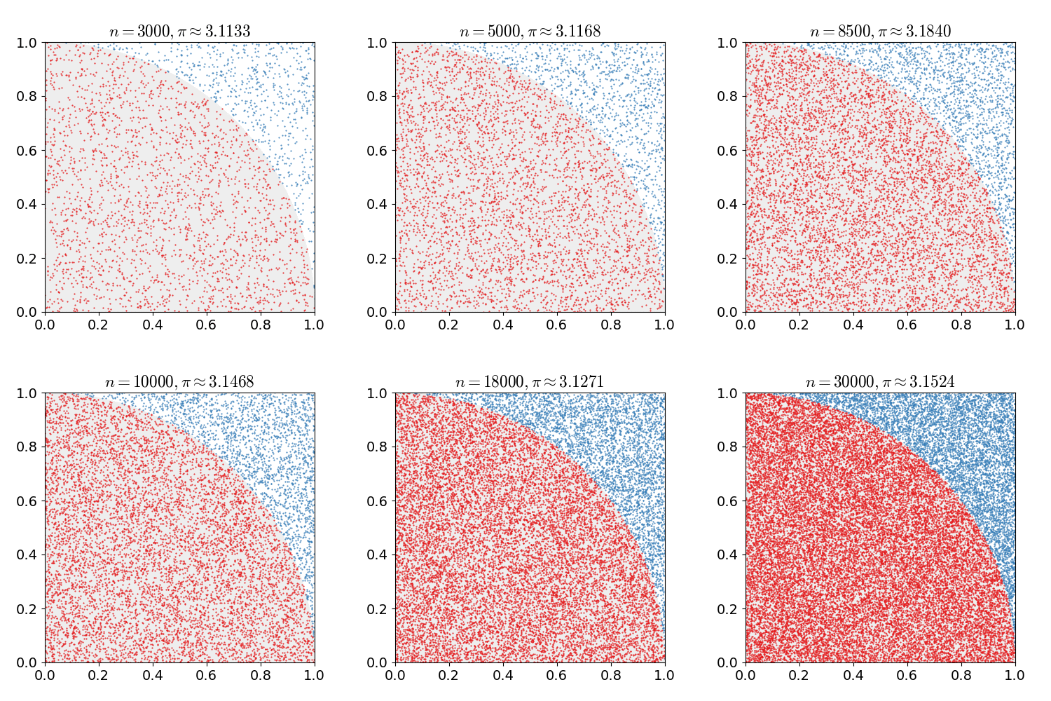
While reading about Monte Carlo methods, I came across this fascinating image created by Caitlin Jo Ramsey:

This plot illustrates a Monte Carlo method for determining π, which I immediately determined to try to reproduce in Python. This post is an IPython Notebook demonstrating how to perform this method using modern Python tools and techniques.
Caveat emptor: Monte Carlo methods are not the best technique for generating approximations of π, so if that's what you are interested in, check out Wikipedia's π page or search around for implementations in your favorite language. On the other hand, the algorithm does offer a nice introduction to Monte Carlo methods as it is
- simple
- reasonably intuitive
- easily verifiable
- fast enough
Let's get started!
Monte Carlo?
What are Monte Carlo methods? A Monte Carlo method is a probabilistic algorithm that relies on random sampling rather than strict determinism to obtain its result. Monte Carlo methods are useful in many fields, particularly when the complexity of the problem in question renders deterministic solutions infeasible.
The example above uses a Monte Carlo method for approximating π. Here's how it works: picture the unit square and the unit circle, with the center of the circle at the origin. Let \(r = 1.0\) be both the radius of the circle and the length of one side of the square, then the area of the quarter-circle inside the square is \({1 \over 4}πr^2\) and the area of the square is \(r^2\), making the ratio of these two areas
\[{{1 \over 4}πr^2 \over r^2} = {π \over 4}\]
A Monte Carlo method for determining π using this knowledge works by
Drawing a set of random points from inside the unit square
Counting the number of points that fall inside the quarter of the unit circle
Calculating the ratio of the number of points inside the quarter of the unit circle to the total number of points, which approaches \(π \over 4\) as the number of random points increases.
This algorithm illustrates the main features of a Monte Carlo method: random (uniformly-distributed) simulation of trials applied over a system that converges as the number of trials increases.
π-ed Python
Implementing this technique in Python is pretty easy, and is greatly aided by the wonderful mathematical and data processing tools available to us in modern Python. As usual, we begin with some imports
from __future__ import division

import math

from matplotlib import pyplot as plt
import numpy as np
import pandas as pd
In order to run the simulation, we need to determine the number of samples we want to use. As you might expect, there is no magical, universally applicable number we can use here: this number represents a trade-off between time and accuracy. How many samples is enough varies widely from problem to problem, but in this case, as I'm more concerned with human understanding than computational accuracy, I've chosen a number that runs fairly quickly on my hardware. After you've read through the post, try changing this number and rerunning the stimulation to see how it affects the results.
n_points = 30000
The first step of the simulation is to scatter random points within the square. numpy makes this step very easy: we simply ask for an \(n \times 2\) array of random numbers, which we then load into a DataFrame. Here are the first 10 points:
df = pd.DataFrame(np.random.rand(n_points, 2), columns=['x', 'y'])
print df[:10]
In or Out
Next we need to determine which points fall within the wedge of the unit circle within the square. How, you ask? Let's ask Pythagoras!
def within_unit_circle(row):
    x, y = row['x'], row['y']
    return math.sqrt(x**2.0 + y**2.0) <= 1.0
That is: given a point inside our square, we know that the point's distance from the origin is given by \(d = \sqrt{x^2 + y^2}\); if $ d ≤ r$, then the point lies within the circle. Neat!
To run this calculation for each of our random points, we can use the DataFrame's apply() method, attaching the result as a new column:
df['within_unit_circle'] = df.apply(within_unit_circle, axis=1)
print df[:10]
The axis=1 argument lets apply() know that we want to apply the function over the rows of the DataFrame, rather than its columns.
Tabulating Truth
Next up: counting. A pandas DataFrame has a sum() method that can be used on its columns. One handy feature of this method is that, when applied to a column of Boolean values, it has the effect of counting the Trues:
boolean_frame = pd.DataFrame({
    'true_blue': [True, True, True],
    'falsehood': [False, False, False],
    'unseemly_fraternization': [True, False, True],
})

print boolean_frame['true_blue'].sum()
print boolean_frame['falsehood'].sum()
print boolean_frame['unseemly_fraternization'].sum()
So, taking sum() for a spin:
df['within_unit_circle'].sum()
Almost π
And just like that, we can compute our approximation of π:
almost_pi = df['within_unit_circle'].sum() / len(df) * 4.0

print almost_pi
print math.pi
print abs(almost_pi - math.pi)
Here is the plot of our data points, shaded like Caitlin Jo's version to distinguish the points inside and outside the wedge:
Keep Calm and π On
Well that was fun! To review, we've
- discussed the basics of Monte Carlo methods
- examined the details of a particular method to approximate π
- used Python's wonderful data manipulation tools to implement the method
Monte Carlo methods are widely used in many different fields, including physics, engineering, and business. To learn more, check out the Wikipedia page on Monte Carlo methods.

No comments:
Post a Comment